


BugStats produces multi-sample environmental summary diagrams from coded habitat data. When used with stratigraphic sequences or repeated pitfall trapping, these diagrams can be used to identify environmental changes through time as reflected in the taxa present in the samples. When used with archaeological samples they can be used to illustrate spatial variation in human impact.
| The method is simple, transparent and uses broad (eco)habitat classifications. Ca. 4995 taxa have been assigned to 22 habitats (BugsEcoCodes, ca. 8317 designations) through a combination of examination of various published habitat descriptions and the detailed ecology codes assigned by Koch (1989-92). 125 Koch codes are included in BugsCEP for ca. 2920 species (ca. 11192 designations), but are yet to be included in graphical outputs. | 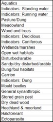 |
|
The categories are based on those most commonly used in Quaternary research, with a little adjustment to cater for archaeological investigations. In particular, the work of the Bugs authors, and Mark Robinson (e.g. 2000), Philippe Ponel (e.g. 1995) and Harry Kenward (e.g. 2001) have influenced the category definitions. The species designations are those of the Bugs authors, with a considerable influence from Klaus Koch's work. Due to the nature of these influences the codes are most likely to be more ecologically useful in Central to Northern Europe. Taxa may be assigned to more than one habitat, but may exist in only one 'indicator' class at a time. |
Despite a probable northern bias the use of a constant system enables reproducibility in any fauna, and thus the system could even be useful where the habitat coding is less accurate.
More information is available in Buckland (2007). The BugsEcoCode system produces quantitative reconstructions from qualitative habitat descriptions/designations. It is thus a reproducible semi-quantitative system which allows advanced inter-site comparisons. Raw and calculated data is always output in the export files, and a sample by sample breakdown of species and their codes and abundances can be obtained.
BugStats is to some extent a work in progress, and we would very
much appreciate feedback on the usefulness and problems with the BugsEcoCode
calculation system and outputs.
| Why BugsEcoCodes & BugStats |
|
| Generate environmental reconstructions for a site & produce BugsEcoGraphs |
| BugStats can produce sample habitat
summary diagrams for any site which includes taxa that have been assigned
BugsEcoCodes. The graphs allow direct comparison of the environments
represented by samples between samples and sites. A number of standardization
and calculation options are available. BugStats uses the concept of environmental representation (env. rep.) as follows: 1 environmental representation = 1 environment represented by 1 individual or taxon. A taxon can represent more than one environment. The raw results are counts of environmental representation in each habitat class for each sample. These can (optionally) be standardized by dividing by the sample sum to allow samples to be compared on a common (percent) scale. |
|
|
|
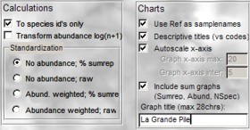 |
Calculations
|
|
||
|
|
|
 |
|
|
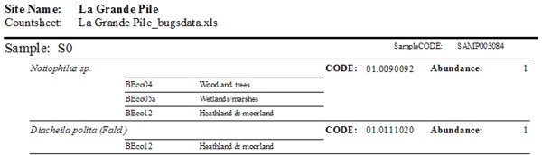
See a sample by sample species breakdown of BugsEcoCodes for a site |
|
The BugStats species breakdown report allows
you to see exactly which represent which environments, and how abundant
they are, in each sample. This is a useful too when trying to understand
the environmental reconstruction diagrams. |
|
 |
|
| Compare samples at a site using correlation coefficients |
|
Correlation coefficients can be used to compare the similarity/dissimilarity of the species composition of samples. This is especially useful when trying to identify samples that represent similar environments in Quaternary geology and environmental archaeology. BugsCEP currently only supports one correlation coefficient - the 'modified Sørensen's' coefficient of similarity of Southwood (1978), which is the inverse (1-B) of the Bray-Curtis coefficient of dissimilarity (Krebs, 1989). Additional coefficients will be added with time. The results are exported as MS Excel files and
can be used as the basis for building cluster diagrams/dendrograms,
but no such feature is present (yet...) in BugsCEP. |
|
| BugStats output files explained |
|
BugStats produces three types of output: |
|
|
BugsEcoGraph files Three worksheets: Graphs; PctResults; RawResults |
|
|
Graphs A horizontal series of 24-27 bar chart like figures (depending on options) as shown below:
The first figure shows sample names and the diagram title provided by the user. The next 23 figures show the BugStats results for each sample in each of the 23 habitat classes of the BugsEcoCode system. Each figure is titled by the class name, and has a scale at the bottom which is either in percent or counts depending on the options chosen. The final three figures provide summary information for each sample if requested. See above for details.
|
|
|
PctResults and RawResults RawResults shows the raw counts of environmental representations
for each sample in each habitat class. 'Indicator' classes are not included in standardization calculations as they are subclasses. The last few columns show sample data, including reference/name, coordinates and depth.
|
|
|
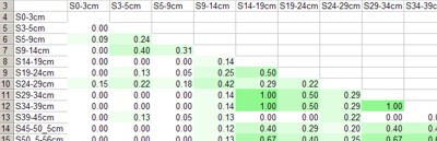
Results are exported as a matrix, with sample names in the first
row and first column. The remaining cells show the coefficient of
similarity values for each sample compared with every other one. A value of 1 represents total similarity, and 0 no similarity. |
 |
|
Tips for improving the graphs for presentation/publication Copy and paste the figures into vector graphics editing software (e.g. CorelDraw)
|
|
|
Please see Buckland (2007) for a detailed description.
|
|
Please see Buckland (2007) for a detailed description.
|
BUCKLAND, P.I. (2007). "The Development and Implementation of Software for Palaeoenvironmental and Palaeoclimatological Research: The Bugs Coleopteran Ecology Package (BugsCEP)". PhD thesis, Environmental Archaeology Lab., Department of Archaeology & Sámi Studies. University of Umeå, Sweden. Archaeology and Environment 23, 236 pp + CD. Available online: http://www.diva-portal.org/umu/abstract.xsql?dbid=1105
KENWARD, H (2001). "Insect remains from the Romano-British ditch terminal at the Flodden Hill Rectilinear Enclosure". Reports from the Environmental Archaeology Unit, York 2001/49, 15pp.
KOCH, K. (1989-92). Die Käfer Mitteleuropas. Ökologie, 1-3. Goecke & Evers, Krefeld.
KREBS CJ, (1989), Ecological methodology. Harper Collins Publishers, New York, USA, p. 654.
PONEL, P. (1995). “Rissian, Eemian and Würmian Coleoptera assemblages from La Grande Pile (Vosges, France)”. Palaeogeography, Palaeoclimatology, Palaeoecology, 114, 1-41.
ROBINSON, M. A. (2001) Insects as palaeoenvironmental indicators. In, D. R. Brothwell & A. M. Pollard (eds.) Handbook of archaeological sciences, 121-133. J. Wiley & sons, Chichester.
SOUTHWOOD TRE, (1978), Ecological methods, with particular reference to the study of insect populations. John Wiley & Sons, New York, 2nd ed., 524p.
